Flywheel Attention: Attention Kernels Built for the TPU

Sep 29, 2026 · Zishuo Bao, Zeshen Zhang, and Yucheng Lu

TPU-native softmax attention and Gated DeltaNet kernels: up to 744 TFLOP/s, 1.56× faster softmax attention and 3.61× faster GDN prefill on TPU v6e.

Code

Attention is all you need. But how much of the hardware can you actually use to run it?

On GPU, attention kernels are a well-studied problem. FlashAttention [1-4] established the fused, tiled, online-softmax formulation that everyone now uses, and every other part of the problem has a well-optimized kernel too: FlashDecode and FlashDecode++ [5] for decode, FlashInfer [6] for serving, and the FLA library [7] for linear attention.

On TPU the hardware is ahead of the software. SemiAnalysis’s InferenceX benchmarks put Ironwood at 50% more tokens per dollar than B200, and the same report notes “substantial work still needed across the software stack” [12]. Attention is a large part of that work. A TPU is a different machine in ways that matter for exactly the attention kernels, and the techniques that make FlashAttention and FLA fast on GPU either do not exist on TPU or point in the wrong direction.

In this post we present Flywheel Attention, a set of TPU attention kernels covering Softmax Attention (MHA, GQA) and Gated DeltaNet (GDN). We compare against the strongest publicly available TPU kernels we know of:

• Softmax attention (MHA, GQA)
  • RPA v3 (rpa_v3) [8]. Ragged Paged Attention v3 is the attention kernel that vLLM’s tpu-inference backend uses for both prefill and decode. It reads keys and values from a paged KV cache and handles a batch of requests with different lengths in a single call, which makes it the kernel that serving on TPU runs through today.
  • Splash Attention (sa) [29]. Splash Attention is the blocked flash attention kernel for TPU maintained in OpenXLA’s Tokamax, and the kernel that MaxText uses for training. It works on dense, fixed-length sequences with block-sparse masks, so it is the natural reference for the forward and backward passes outside of serving.
• Gated DeltaNet
  • GDN v3 (gdn_v3) [30]. gdn_v3 is the Gated DeltaNet Pallas kernel shipped in tpu-inference for hybrid models such as Qwen3-Next, covering the chunked prefill pass and the recurrent decode step. As far as we know it is the only GDN kernel for TPU in public use.

On TPU v6e, our softmax attention forward reaches 744 TFLOP/s at head dimension 256, 81% of the chip’s BF16 peak, and is up to 3.49× faster than rpa_v3 and up to 1.56× faster than sa. Our GDN prefill kernel is up to 3.61× faster than gdn_v3. In tpu-inference, the kernels speed up end-to-end time for long-context applications such as video understanding and document retrieval.

Note: throughout this post, “GPU” means NVIDIA Hopper (sm90) and later, and “TPU” means TPU v6e unless a generation is named. The constraints in Section 2 hold across TPU generations, so the analysis carries over to earlier chips and to Ironwood with the tile and MXU sizes adjusted.

1. How attention runs on a GPU today

We start from what the two kinds of attention compute, and how GPU kernels compute them fast. We keep the notation to the minimum and drop constants like the gates, scale factors and masks. The full formulations are in the FlashAttention paper [1] for softmax attention and in [10, 11] for Gated DeltaNet.

Softmax attention. For one head, query $Q$, key $K$ and value $V$ have one row per token, and

\[P = \text{softmax}(Q K^\top), \qquad O = P V\]

FlashAttention [1] never builds the full $P$ matrix. It walks over blocks of $K$ and $V$ and keeps three running values per query row: the largest score so far $m$, the sum of exponentiated scores $l$, and the output accumulator $o$. When a block arrives with scores $s$,

\[m' = \max(m, \max s), \qquad p = e^{s - m'}, \qquad l \leftarrow e^{m - m'}\, l + \textstyle\sum p, \qquad o \leftarrow e^{m - m'}\, o + p\,V\]

and the output is $o / l$ at the end. The factor $e^{m - m’}$ is the rescale: whenever a block raises the running max, everything accumulated so far is rescaled to incorporate that max value.

On GPU this loop has been tuned for four generations. FlashAttention-2 [2] split the work across warps so that none waits on another. FlashAttention-3 [3] separated the threads that load tiles from the threads that compute on them, and let two compute groups alternate so that one’s softmax overlaps the other’s matmuls. FlashAttention-4 [4] skips the rescale when the max barely moves. Serving kernels such as FlashInfer [6] walk a paged, ragged KV cache with plain pointer arithmetic.

Gated DeltaNet. GDN [10] replaces the growing KV cache with a fixed-size state $S$ per head, which every token updates with a decay and a write strength $\beta$. Kernels process chunks of $C = 64$ tokens at once [11]. For one chunk, with $Q$, $K$, $V$ its rows and the gates folded in:

\[A_{kk} = \text{lower}(K K^\top), \qquad A_{qk} = \text{lower}(Q K^\top), \qquad V_\text{new} = (I + A_{kk})^{-1}(\ldots) - (\ldots)\,S\] \[O = Q S + A_{qk} V_\text{new}, \qquad S \leftarrow S + K^\top V_\text{new}\]

where $\text{lower}$ keeps the lower-triangular part and the elided terms are $V$ and $K$ with the gates applied. Everything here is a matmul except the inverse of a $64 \times 64$ lower-triangular matrix $(I + A_{kk})^{-1}$. Before the delta rule, the qkv projection (width $\text{dim} = 2 n_{kq} d_k + n_v d_v$) goes through a 4-tap causal convolution along the token axis, and $Q$ and $K$ are l2-normalized. A layer has $n_{kq}$ query/key heads shared by $n_v$ value heads.

The GPU kernels for this loop live in the FLA library [7]. They do the triangular inverse by forward substitution on the CUDA cores and the convolution, gates and normalizations as ordinary elementwise code, all of it a rounding error next to the matmuls on a GPU.

2. Why the GPU playbook does not transfer to TPU

Everything in the previous section rests on four things a GPU provides:

• Loads that pull strided tiles out of a tensor in whatever layout it already has, through TMA or plain pointer arithmetic [18];
• Tensor cores that read both operands with every instruction, from shared memory, registers or tensor memory, with no separate weight-load step [28];
• Vector units that run concurrently with the tensor cores [3];
• Many resident warps, and a hardware warp scheduler that switches among them to hide latency [13, 14, 15].

A TPU TensorCore has none of these, or at least, not in the same form. It is an in-order VLIW machine: a single-threaded scalar unit fetches VLIW bundles, executes their scalar slots and forwards the rest to the vector and matrix units. A separate asynchronous DMA unit moves data between HBM and VMEM [19, 20]. Vector and matrix work does issue in parallel, but only as far as the compiler packed it into the same bundles. The four GPU capabilities above become four constraints for TPUs, and each one shows up directly in an attention kernel.

Layout is not the kernel’s to choose. From TPU v2 through v6e a vector register holds an 8×128 tile of 32-bit values, 16×128 once BF16 is packed two rows per word, and the last two dimensions of any array are the ones that land on it. Ironwood widens the register to 16×256 [20, 22, 27]. The last two dimensions of a block shape must be divisible by 8 and 128, or equal the full array [22]. In HBM, XLA stores BF16 arrays in 8×128 tiles with pairs of rows packed into one 32-bit word [21], which is why a DMA window into an activation starts on an 8-row grid.

Weight-stationary MXUs. A TensorCore holds a small number of MXUs: four 128×128 systolic arrays on v4, v5e and v5p, two 256×256 arrays on v6e, and two 256×256 arrays on Ironwood [20, 23]. Each MXU takes a matmul in two steps: push the right-hand operand into the array, then stream the left-hand rows through it and pop the results from a FIFO [24, 25]. Pushes, matmuls and pops are all slots in the core’s single instruction stream, so the compiler’s schedule serializes them [19, 25].

A narrow vector side. In addition to MXU, we have a VPU for elementwise work, an EUP for transcendentals such as exp, and an XLU for transposes and permutes [22, 24, 26]. Each bundle has a fixed number of slots per unit [19, 20]. The vector math, loads and stores fill it and every register spill compete for the same few slots of a single instruction stream.

No fine-grained hardware scheduler. Mosaic, the compiler behind Pallas on TPU, performs layout inference and lowering and emits MXU, VPU, EUP and XLU work in program order [26, 27]. The LLO scheduler then reorders independent instructions within a basic block and packs them into bundles [22, 26]. The compiler can overlap some vector and matrix work, but that overlap is limited by the dependency graph the kernel exposes. Within one step of an attention loop, QK feeds exp and exp feeds PV, so the independent work that could fill the gaps sits in other steps, and runtime loop boundaries can still drain the pipeline. Any overlap beyond that is the kernel’s to write.

Table 1 takes one technique from Section 1 for each constraint and shows where it breaks.

Table 1. One GPU attention technique per constraint, and why it fails on TPU.

Constraint	What works on GPU	Why it fails on TPU
Layout is not the kernel’s to choose	The kernel reads Q, K, V in the model’s own layout, and a ragged sequence starts at any token via TMA or pointer arithmetic.	Any other layout could easily be a full HBM pass outside the kernel, and a sequence cannot start off the 8-row grid.
Weight-stationary MXUs	Tensor cores are fed from registers by many warps; operand reuse can reduce data movement, with mechanisms that depend on the GPU architecture and MMA instruction.	Every matmul begins with a push, and an operand pushed twice, or transposed, spends MXU slots nothing else can use. Reusing the resident right-hand operand amortizes the MXU weight-push cost across matmuls.
A narrow vector side	Softmax and the delta rule’s solve, convolution and gates run as ordinary vector code on CUDA cores and SFUs, hidden behind the matmuls.	The vector slots saturate first.
No fine-grained hardware scheduler	Concurrent warpgroups, interleaved by the warp scheduler, so one group’s softmax overlaps another’s matmuls (FA3).	One instruction stream. The compiler can reorder independent instructions, but overlap is limited by the program’s dependency graph; runtime loop boundaries can still drain the pipeline.

3. The Flywheel kernels

The Flywheel kernels are our answer to the four rows of Table 1, together with the observation that one answer per row serves both forms of attention. Table 2 summarizes how Flywheel Attention addresses the four constraints on TPUs.

Table 2. An overview of Flywheel optimizations.

TPU Constraint	Softmax attention (MHA, GQA)	Gated DeltaNet
Layout is not the kernel’s to choose	Tokens on sublanes: one head per block, ragged sequences snapped to the 8-row grid with an output copy.	Native layout in, packed output out: [T, dim] BF16 in, [T, n_v·d_v] out, no XLA retile or upcast.
Weight-stationary MXUs	Long query blocks stream through each pushed key and value tile, and the fragment pipeline keeps the next push in flight.	Push each weight once: $K^\top$ shared by $A_{kk}$ and $A_{qk}$, $V_\text{new}$ shared by output and state update, they are never transposed. We issue two heads per push.
A narrow vector side	Static-anchor softmax: no running max, no rescale, one check per block; scores in log2 units.	Vector work onto the MXU: triangular inverse as 8 BF16 matmuls, convolution as one matmul against a constant selector, silu and l2norm at one EUP push each.
No fine-grained hardware scheduler	A pipeline across fragments: fully unrolled, spanning every head in the block.	Fill the gaps: other chunks’ matmuls emitted into the inverse’s 200-cycle latency gaps.

3.1 Softmax Attention (MHA and GQA)

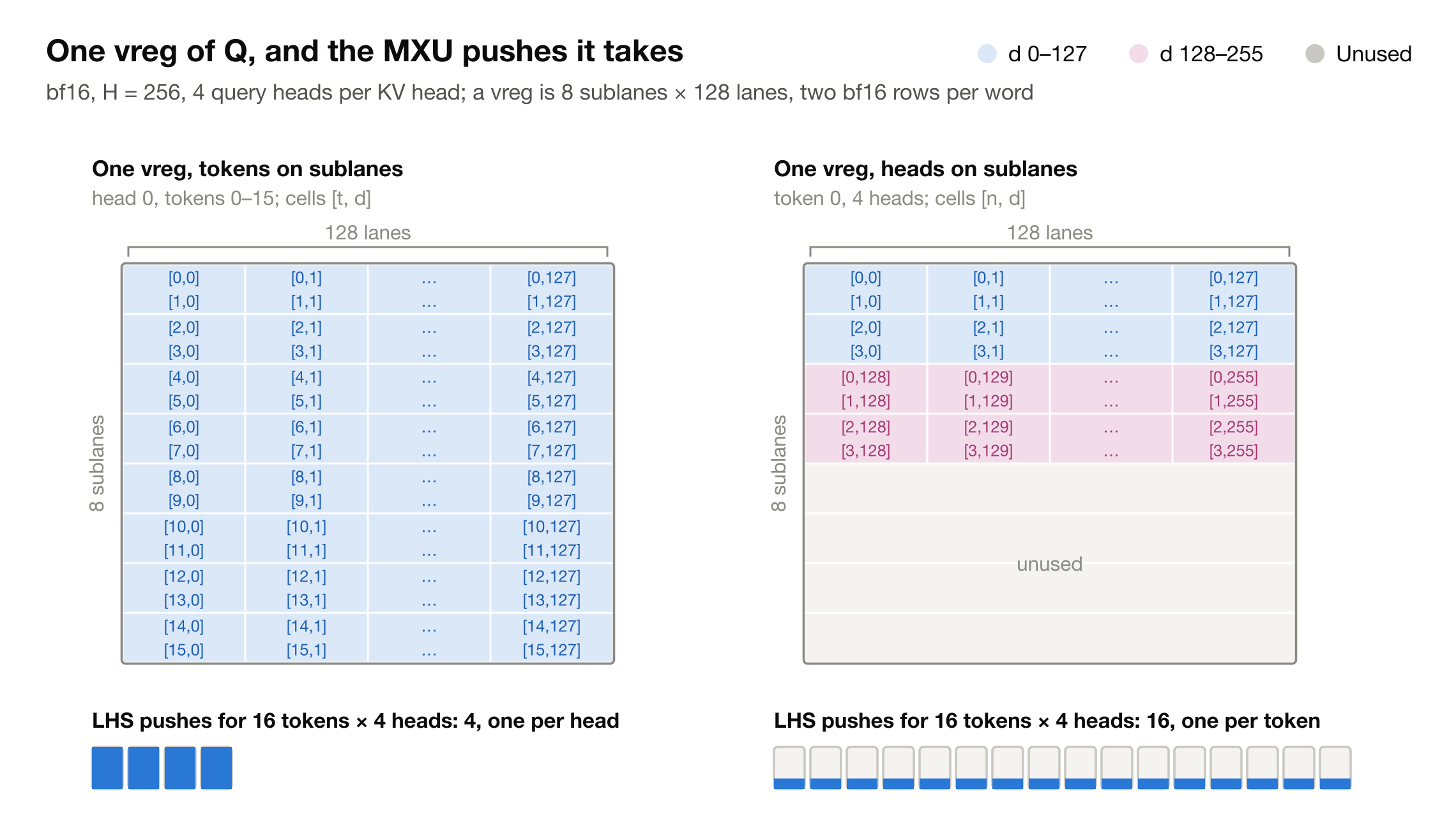
Figure 1. Tokens on sublanes (ours, left) vs. heads on sublanes (rpa_v3, right): each head becomes a dense [T, D] tile, and 16 tokens × 4 heads take 4 MXU pushes instead of 16.

Tokens on sublanes. The first problem is the layout constraint. Omitting the batch dimension, an attention input is a [T, H, D] array of sequence length, heads and head dimension. $D$ goes on lanes in any sensible layout, so the one real choice is what goes on sublanes. rpa_v3 keeps the model’s order and puts heads there. Tokens then sit on a leading axis, where a ragged sequence can start at any token, but every query block carries all the heads of its tokens, and so do its $m$, $l$ and $o$. We see the issue with this design choice is that the more heads on a chip, the shorter the blocks, and every extra block re-reads $K$ and $V$. We instead put tokens on sublanes, as [H, T, D]and let the “reshape” fuse with the RoPE after. A [T, D] tile is exactly an MXU operand, every DMA moves whole tiles, and a block belongs to a single head, so its length no longer depends on how many heads the model has. GQA needs no stacking of query heads either: query head $h$ simply reads KV head within that group.

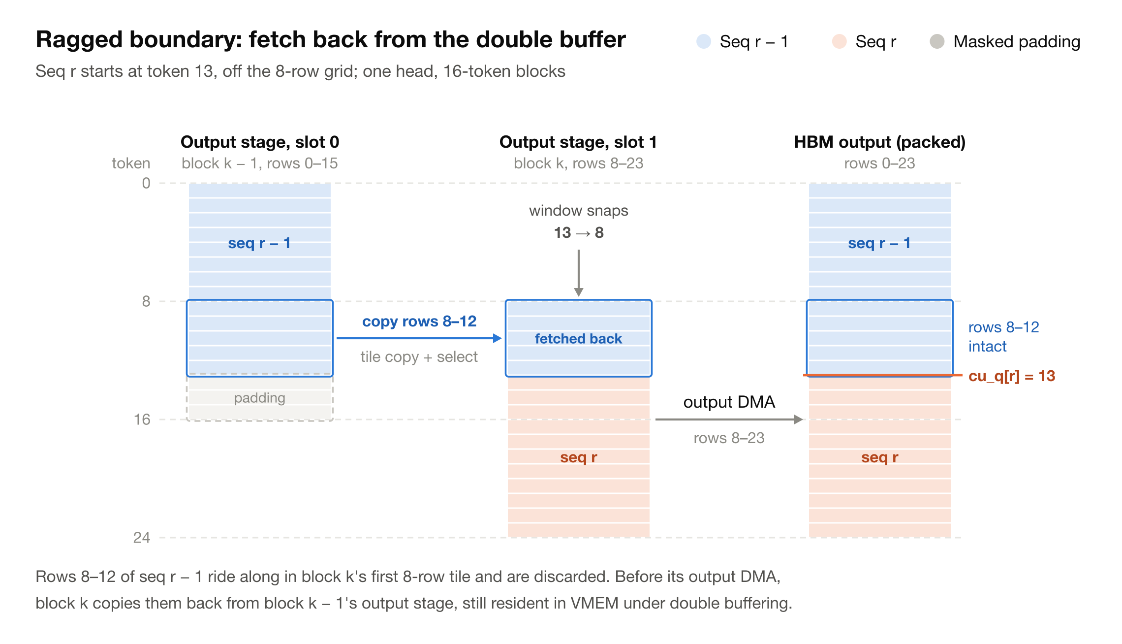
Figure 2. Seq r’s window snaps from row 13 down to row 8. Rows 8–12 of seq r − 1 are copied back from block k − 1’s output stage in VMEM before the output DMA.

We pay for this in two places.

• Inside the kernel, a sequence’s DMA window can only start on the 8-row grid. We snap each window’s start down to a multiple of 8, so up to 7 rows of the previous sequence ride along at the top of its first block. Before the output DMA we copy those rows back from the previous block’s output, which double buffering keeps in VMEM, and the block lands directly in its final place in the packed output. This is 1.9–3.0× faster on ragged batches than a padded write followed by a gather.
• Outside the kernel, the layout costs nothing. Q, K and V come out of the QKV projection on the hidden states, and XLA writes them in [H, T, D] directly; the per-head norms and K’s RoPE read and write that layout. Q’s RoPE moves into the kernel and is applied in FP32 to each Q tile after its DMA lands. The output projection reads the kernel’s [H, T, D] output as is, so the compiled HLO has no transpose or copy between the hidden states and the output projection.

Static-anchor softmax. Online softmax rescales the whole accumulator whenever the running max moves. FlashAttention-4 skips the rescale when the max barely moves, but on TPU tracking and comparing the max on every fragment cost as much as the rescales it saved and spilled our pipeline to VMEM. We propose using a static-anchor version. Our key insight is that the anchor does not have to be the max, only close enough that nothing overflows. So each row fixes its anchor at the max of its first fragment and never moves it:

# Online softmax: rescale on every fragment
m_new = maximum(m, rowmax(s))
alpha = exp(m - m_new)
l = alpha * l + rowsum(exp(s - m_new))
o = alpha * o + exp(s - m_new) @ v

# Static anchor: fast path, no rescale
p = exp2(s - anchor)
l = l + rowsum(p)
o = o + p @ v

Rather than check scores, we check the running sum once per block: it includes every exponentiated score, so a small sum proves no score crossed the line. A block that fails sets a flag in scalar memory and is replayed with the rescaling softmax. We have seen the literature does something similar before: Tokamax Splash Attention (sa) [29] exposes a related fixed-anchor path through max_logit_const: the caller supplies one constant, and the kernel uses it in place of the running maximum for every row. That moves the burden to the user, who must know a safe bound for the model’s logits before the call.

Our static anchor differs on each point. The anchor is chosen inside the kernel from the first fragment’s maximum, so the caller supplies nothing and no offline calibration is needed. The kernel then verifies its own guess: after each block it checks that the running denominator stays within the FP32 budget, raises a flag in SMEM if the check fails, and replays that row block with the standard online softmax. The result is therefore exact for any input, and the fast path is taken whenever the check passes, which in practice is nearly always. Appendix A gives the failure analysis. With scores kept in log2 units, every exp is an exp2 with no per-score multiply. The static anchor alone is worth 25–40% of forward throughput at head dimension 256.

A pipeline across fragments. TPU compilers can overlap some vector and matrix work, but we found that relying on instruction scheduling alone leaves the available overlap constrained by the structure exposed by the kernel. rpa_v3 explicitly writes the schedule by hand: it interleaves one KV head’s QK-plus-softmax with the previous head’s PV. The limitation is that the pipeline depth is therefore tied to the number of KV heads resident on each chip. Under GQA with high tensor parallelism, this can collapse to a single head, leaving no head-level work to overlap. Moreover, the pipeline sits inside a runtime loop over KV chunks, so it drains and refills at every chunk boundary.

We move the overlap down to the KV fragments within a head: each fragment’s QK and exp2 are emitted right next to the previous fragment’s PV, fully unrolled, spanning every fragment of every head in the block:

probs = softmax(qk(frag[0]))
for i in range(1, num_fragments):       # fully unrolled
    next_probs = softmax(qk(frag[i]))   # MXU: QK of i, VPU/EUP: exp2 of i
    pv(frag[i - 1], probs)              # MXU: PV of i - 1
    probs = next_probs
pv(frag[-1], probs)

The pipeline also keeps the MXU’s push queue full: the next fragment’s push is issued while the previous fragment’s result is still draining.

3.2 Gated DeltaNet

Native layout in, packed output out. The layout constraint costs gdn_v3 more than it costs rpa_v3. gdn_v3 wants [T, 1, dim] in FP32 so the convolution’s 4-token shift is register naming; producing it costs an XLA retile and upcast. We take the qkv projection in the caller’s [T, dim] BF16 layout, cast on chip, and write packed output with the same 8-row snapping and copy as the softmax kernel.

Vector work onto the MXU. Three things in the GDN kernel will saturate the vector units, and this is where the narrow vector side costs GDN the most: the triangular solve, the convolution and the activations. In Flywheel, we move entirely these vector work onto the MXU with transformation below.

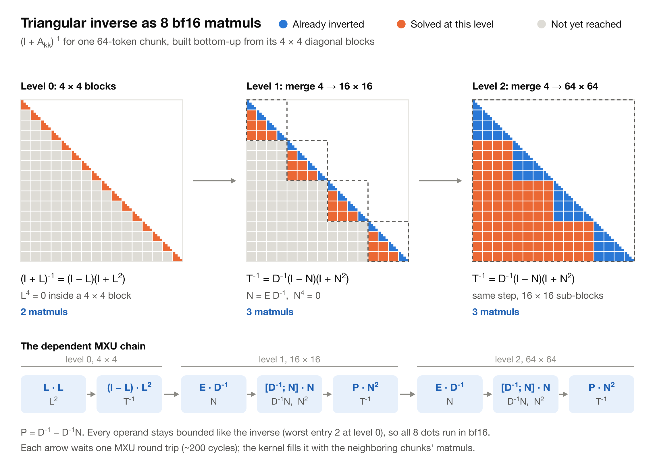
Figure 3. Triangular inverse as 8 BF16 matmuls, built bottom-up from the 4×4 diagonal blocks of one 64-token chunk.

The triangular inverse. gdn_v3 inverts $I + A_{kk}$ by forward substitution on the VPU, 64 dependent steps per chunk. Since a strictly lower-triangular $L$ has $L^{64} = 0$, the inverse is a product of matmuls, $(I - L)(I + L^2)\cdots(I + L^{32})$ [9]. On the whole chunk this will lead to incorrect results: with repeated keys the powers hold binomial sums near $10^{17}$ that cancel only at the end. Flywheel inverts the $4 \times 4$ diagonal blocks first, where the worst intermediate is 2, then merge four at a time with the same expansion at block level, 4 → 16 → 64 (Figure 3):

\[T = D + E, \qquad T^{-1} = D^{-1}(I - N)(I + N^2), \qquad N = E D^{-1},\ N^4 = 0\]

Every intermediate stays bounded like the inverse itself, so all 8 matmuls run in BF16 with a max error of $9 \times 10^{-3}$ on repeated keys. We note that Tokamax’s KDA kernel already replaces this serial solve with a matrix-multiplication formulation based on the nilpotence of the strictly lower-triangular part. The main contribution here with Flywheel is therefore not the math, but how the inverse is decomposed to make that algebra numerically viable in BF16.

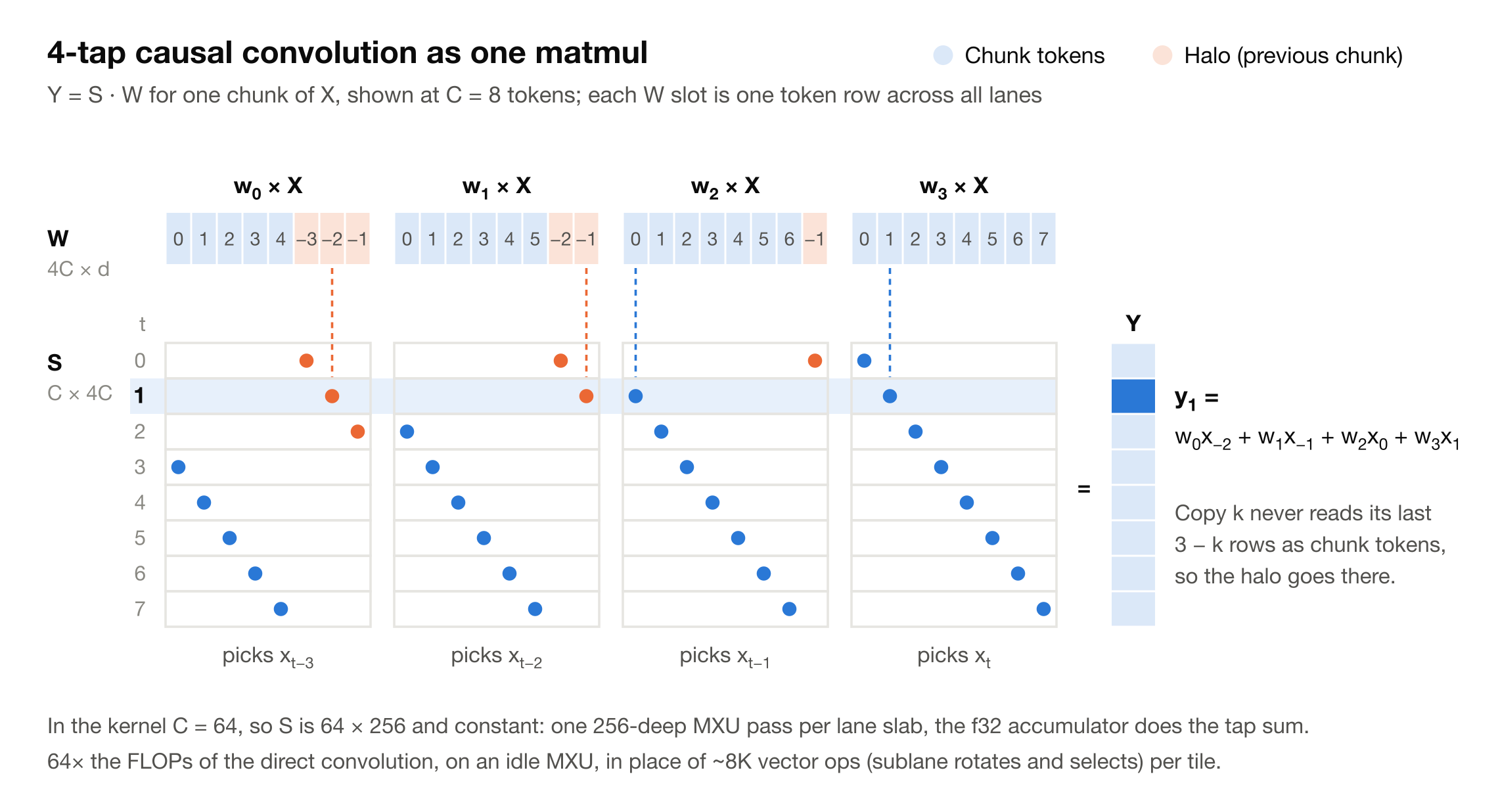
Figure 4. 4-tap causal convolution as one matmul against a constant 0/1 selector.

The convolution. GDN applies a short causal convolution (4 taps) along the token axis before the recurrence. With tokens on sublanes, shifting the sequence by one token is a sublane rotate followed by a select, and the four shifts add up to about 8K vector operations per tile, all on the units that are already the bottleneck. We move this work to the MXU instead. A causal convolution is a matrix multiply by a banded matrix, so we write the four shifted copies as one stacked operand, scale each copy by its tap weight, and multiply by a constant 0/1 selector matrix built at compile time that picks out the right row from each copy (Figure 4). The MXU’s FP32 accumulator does the sum. This costs 64× the FLOPs of the direct convolution, but they run on a unit that was idle, and the vector work disappears entirely.

Activations. Two elementwise functions in GDN each need two transcendental evaluations when written the obvious way. We rewrite them so each needs one: silu as $0.5\,x\,(1 + \tanh(x/2))$, which uses one tanh instead of an exp and a divide, and l2norm as $x \cdot \text{rsqrt}(\sum x^2)$, which uses one rsqrt instead of a sqrt and a divide. Each saves one EUP push per element, about 4% per tile.

Push each weight once. With the inverse and the convolution moved onto the MXU, the MXU itself became the bottleneck. So we reduced the number of pushes in three ways.

• Share K across two matmuls. Both $A_{kk} = K K^\top$ and $A_{qk} = Q K^\top$ use $K^\top$ as the weight. We transpose K once per head group on the XLU, stack Q under K as one left-hand operand $[K;\,Q]$, and compute both products with a single push of $K^\top$. The transpose is done in FP32 on purpose: in BF16, Mosaic recognizes the pattern and folds it back into a transposed push, which costs about twice as much as a normal one.
• Share $V_\text{new}$ the same way. The output and the state update both multiply by $V_\text{new}$, so they share one push.
• Two heads per push. A head’s weight is 128 wide and the v6e MXU is 256 wide, so we place two heads side by side as a block-diagonal weight and stream both heads’ inputs through one push.

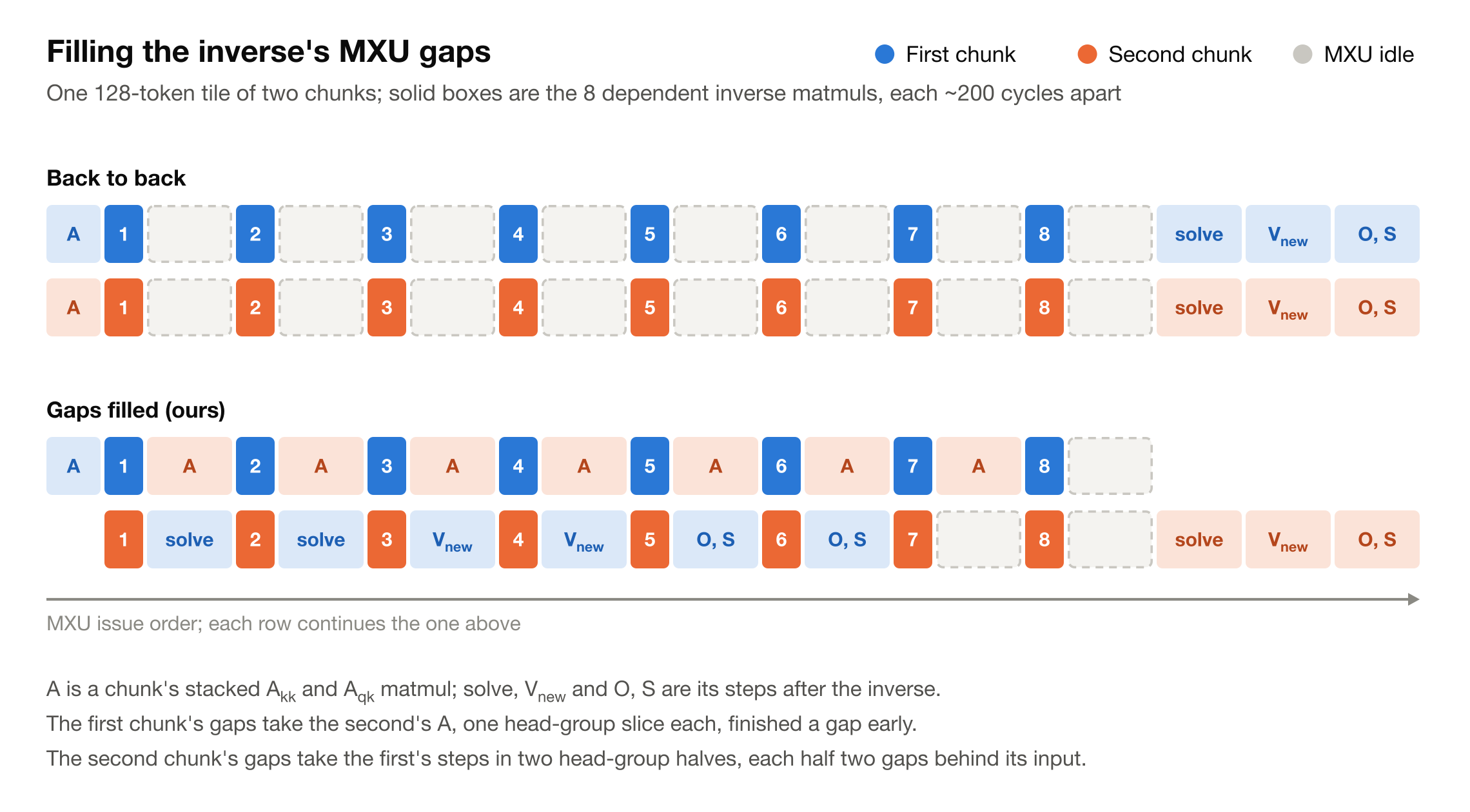
Figure 5. Filling the inverse’s MXU gaps in one 128-token tile of two chunks; the 8 dependent inverse matmuls are about 200 cycles apart.

Fill the gaps. After the push count came down, the remaining waste was latency. Each MXU matmul takes about 200 cycles to return its result, and the inverse is a chain of 8 matmuls where each one needs the previous result before it can start, so the MXU sits idle for most of that chain. On a GPU the hardware scheduler would fill those idle cycles with work from other warps; on TPU nothing does this for us (constraint 4), so the kernel has to interleave the work itself.

The idle cycles are filled with matmuls from neighboring chunks that do not depend on the inverse in progress. A tile holds two chunks. While the first chunk’s inverse runs, we issue the second chunk’s $A_{kk}$ and $A_{qk}$, which need only that chunk’s K and Q. While the second chunk’s inverse runs, we issue the first chunk’s triangular solves, output and state update, whose inverse is already complete. In code this is a callback attached to each matmul of the inverse chain: after the matmul is emitted, the callback emits one independent matmul, so each independent operation lands two positions behind the inputs it needs (Figure 5).

4. Results

We measure the Flywheel kernels at two levels: kernel-level speedup against the production kernels in isolation, and engine-level speedup inside vLLM’s tpu-inference (commit 4420cae) on long-context applications, including needle-in-a-haystack retrieval, multi-hop reasoning over long documents, and video understanding. All runs are on TPU v6e. Each v6e chip has one TensorCore with two 256×256 MXUs and a BF16 peak of 918 TFLOP/s; kernel-level numbers use one chip, and engine-level numbers use a v6e-8 at TP8 for contexts up to 256K and a v6e-16 at TP8 with prefill context parallelism 2 at 512K.

4.1 Kernel level

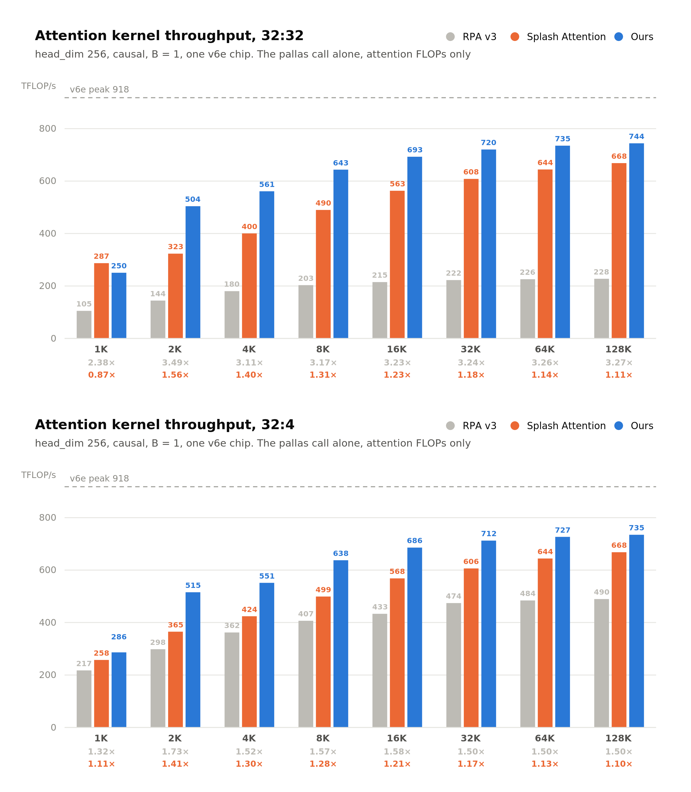
Figure 6. Softmax attention forward throughput at head dimension 256 on one v6e chip: MHA (top) and GQA with 8 query heads per KV head (bottom). The numbers under each length are our speedup over rpa_v3 (grey) and sa (orange).

Figure 6 runs the forward at head dimension 256, causal, batch 1 on one v6e chip, with 32 query heads and either 32 KV heads (MHA) or 4 (GQA, 8 query heads per KV head), and times the attention kernel alone. Under MHA ours reaches 693 TFLOP/s at 16K and 744 TFLOP/s at 128K, 81% of the chip’s BF16 peak. Against rpa_v3 with its tuned block sizes it is $2.4\text{–}3.5\times$ faster under MHA and $1.3\text{–}1.7\times$ under GQA. Against sa, whose block sizes are tuned per sequence length, it is $1.1\text{–}1.6\times$ faster from 2K on, and the gap narrows as sequences grow; at 1K under MHA sa is 15% faster. Our throughput barely depends on the number of KV heads: from 8K on, MHA and GQA are within about 1% of each other, and sa behaves the same way. rpa_v3 is the opposite. It keeps heads on sublanes, so its blocks shrink as KV heads are added, and at 128K it drops from 490 TFLOP/s with 4 KV heads to 228 with 32. These are kernel-only timings, which if anything favour rpa_v3: its input shape needs extra layout work before the kernel runs, and Appendix B measures that on the whole attention block.

For GDN prefill we time the whole fused_conv1d_gdn call on v6e including XLA glue, with BF16 qkv, 16 query/key heads, head dimension 128, and 1 or 8 equal-length sequences packed into one call (Figure 7).

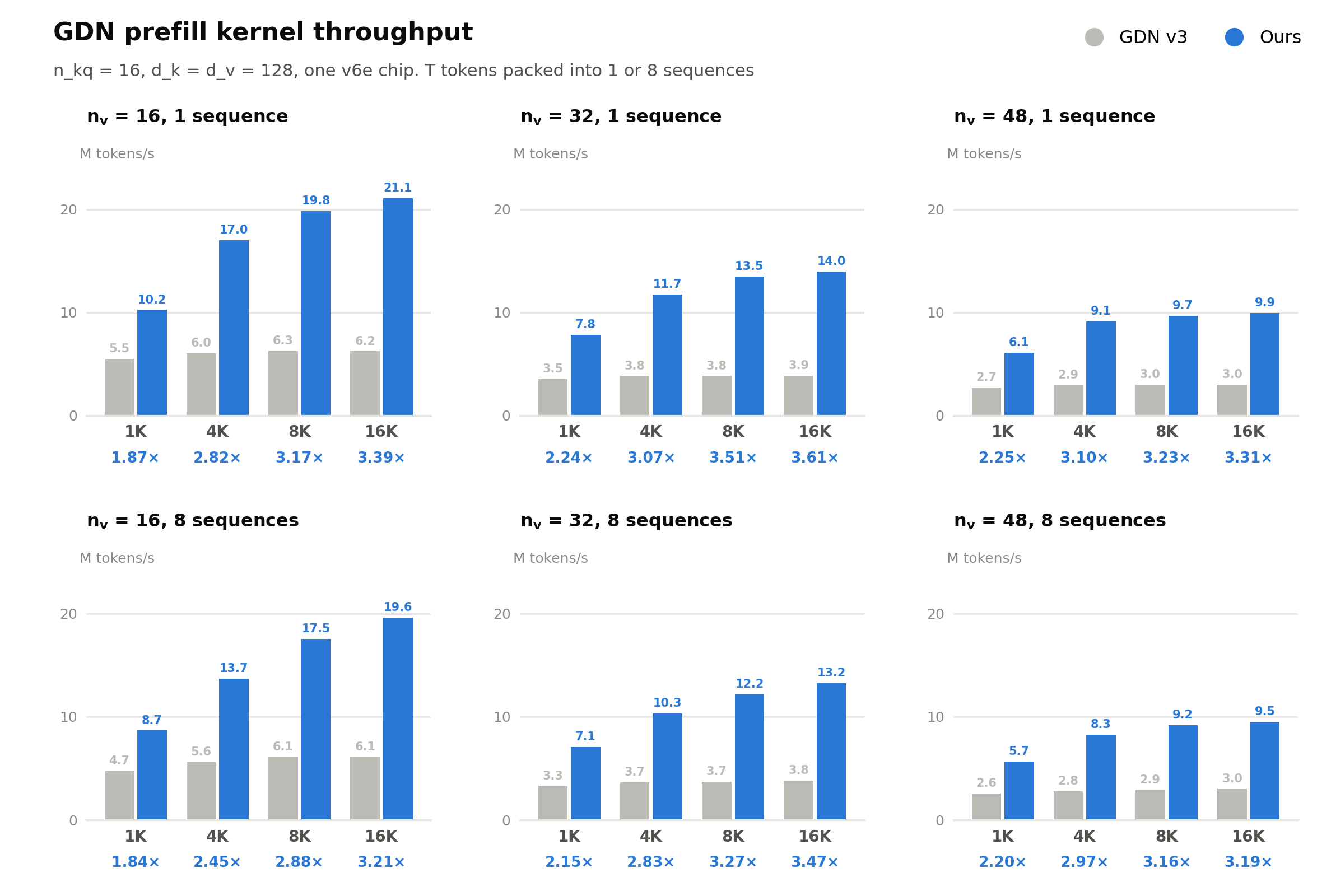
Figure 7. Fused conv1d + GDN prefill on one v6e chip, 16 q/k heads, head_dim 128, T tokens packed into 1 or 8 sequences. The row under each T is our speedup over gdn_v3.

The speedup is 1.8–2.2× at 1K tokens, 2.5–3.1× at 4K and 2.9–3.6× from 8K on. At 8K the largest single steps were the native layout (about 1.4×), the MXU inverse (1.21×), the convolution on the MXU (20% per tile) and the packed output (14%).

4.2 Application level

Kernel speedups do not always survive a serving stack, so we ran both kernels inside tpu-inference (commit 4420cae) on a model that exercises both. Qwen3.8-27B interleaves GDN layers with softmax attention at roughly 3:1. Its softmax layers use head dimension 256 with 24 query heads and 4 KV heads; its GDN layers have 48 value heads. We swap in both of our kernels and change nothing else. Runs up to 256K use a v6e-8 at TP8; the 512K run uses a v6e-16 at TP8 with prefill context parallelism 2.

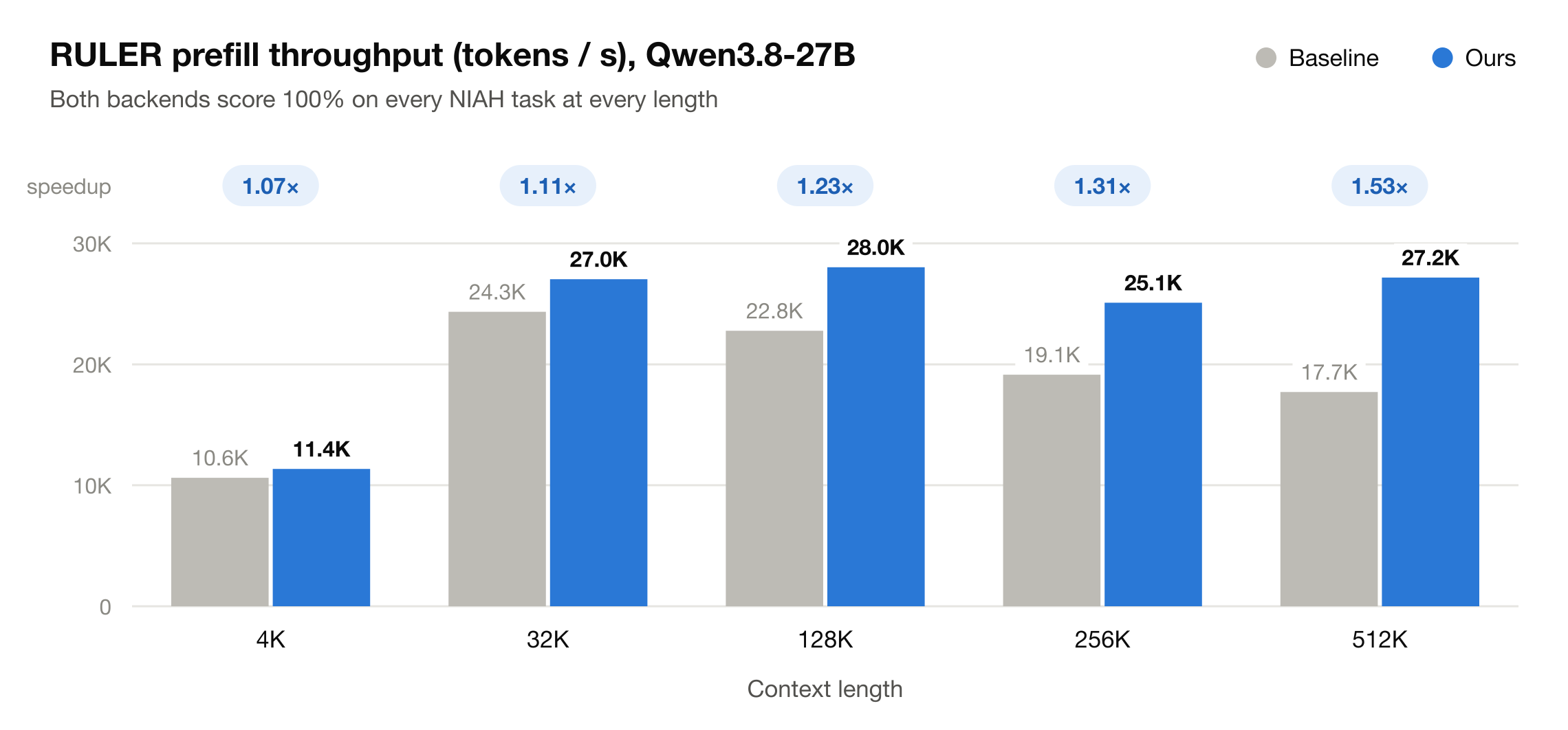
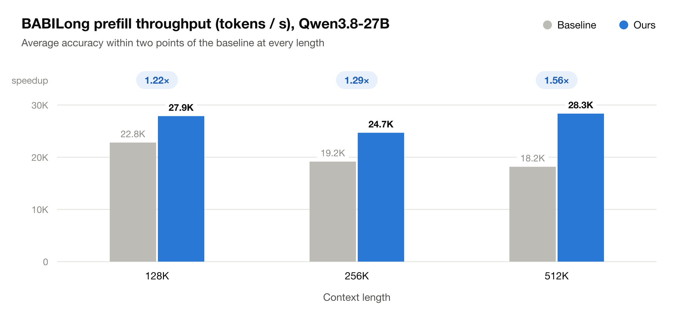
Figure 8. Prefill throughput of Qwen3.8-27B in vLLM, baseline vs ours: RULER (top) and BABILong (bottom).

Figure 8 shows the results. On RULER’s needle-in-a-haystack tasks both backends score 100% at every length. Prefill throughput is 1.07× at 4K, 1.23× at 128K and 1.53× at 512K. BABILong at 128K, 256K and 512K shows 1.22×, 1.29× and 1.56×, with average accuracy within two points of the baseline at every length.

Why are the end-to-end gains smaller than the kernel gains, and why do they grow with context? This can be explained by the Amdahl’s law. At 4K most of a prefill step goes to the projections and the MLP, and attention is a small slice of it. As the context grows, softmax attention grows quadratically and takes over the step. Video-MME shows the split directly below.

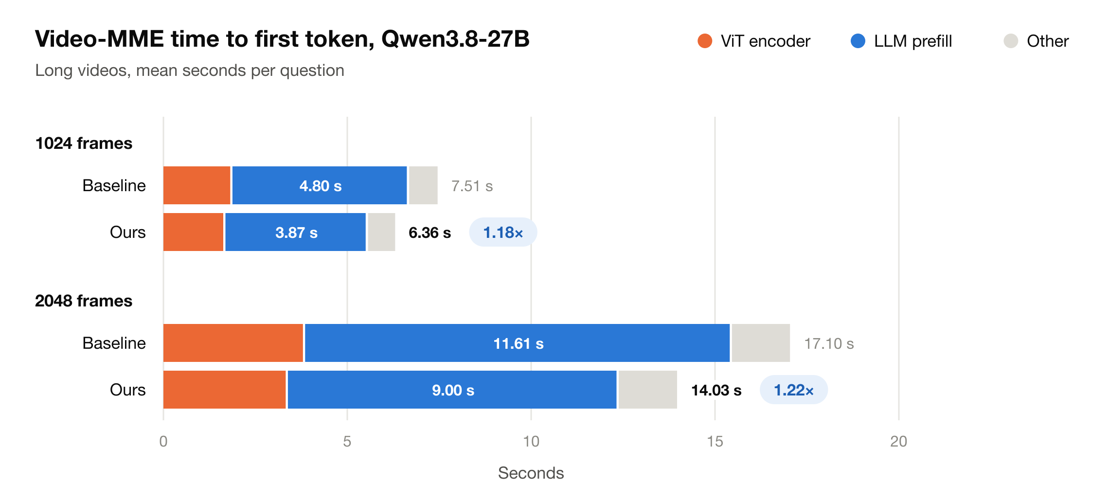
Figure 9. Video-MME time to first token on long videos, split into ViT encoder, LLM prefill and other.

On long videos, the LLM prefill segment gets 1.24× faster at 1024 frames (4.80 s to 3.87 s) and 1.29× at 2048 frames (11.61 s to 9.00 s). The vision encoder and everything else change little, so time to first token improves 1.18× and 1.22×. Accuracy is unchanged: 71.5 vs 71.7 at 1024 frames, 70.6 vs 70.6 at 2048.

5. Limitations and what’s next

What the kernels do not cover yet

• GDN decode and speculative verification still run gdn_v3’s token-recurrent math. Only their I/O moved to the native layout.
• Softmax attention decode is at parity with rpa_v3, not ahead of it. At decode the KV read is the bound either way, and the layout and pipeline work of Section 3 buys little there.
• Hybrid models with MLA layers, such as Ling-3.0, only benefit in their linear-attention layers. The MLA layers are untouched and dominate the step at long context, which is why the speedup on that model falls from 1.8× at 1K tokens to 1.05× at 64K.

Hardware and scale

• Everything so far is on v6e. Our v7x tuning is in progress; its 16×256 vector registers and 256×256 MXUs change the tile geometry in Section 2, but we expect the layout decisions to carry over.
• Context parallelism currently uses a naive all-gather. At 8K tokens the gather dominates and the kernel cannot help; we will explore other alternatives like a ring-style schedule next.

6. Acknowledgement

This work was supported by a 2026 Google TPU Research Award. We gratefully acknowledge Google for its generous support, with special thanks to the TPU Builders Program. We would also like to extend our sincere thanks to Josh Gordon, Lauren Jensen, and Karan Bal for their support throughout the project.

Appendix A: Why the static anchor is safe

Setup. Fix one query row. Let $s_1, \ldots, s_N$ be its scores against the $N$ keys it attends to, in natural-log units (the kernel works in log2 units, which rescales every exponent below by the same constant). Let $a$ be the row’s anchor, the largest score in its first fragment, so $a$ is itself one of the $s_j$. The fast path computes

\[p_j = e^{s_j - a}, \qquad l = \sum_j p_j, \qquad o = \sum_j p_j v_j\]

accumulated in FP32, whose largest finite value is about $e^{88.7}$. Assume every entry of every $v_j$ has magnitude at most $V_{\max}$; the kernel budgets $V_{\max} = 2^{12}$. Define

\[\tau = 88.7 - \ln N - \ln V_{\max} - \delta\]

with a safety margin $\delta > 0$; the kernel uses $\delta = 2$ nats and refuses any configuration where $\tau < 20$ nats.

Claim 1 (no overflow). If $s_j - a \le \tau$ for every $j$, then $l$ and every entry of $o$ stay below $e^{88.7 - \delta}$ throughout the accumulation.

Proof. Each $p_j \le e^\tau$, so every partial sum of $l$ is at most $N e^\tau = e^{88.7 - \ln V_{\max} - \delta} < e^{88.7 - \delta}$. Every entry of every partial sum of $o$ is at most $\sum_j p_j \lvert v_j \rvert \le V_{\max} \cdot l \le N e^\tau V_{\max} = e^{88.7 - \delta}$. ∎

For $N = 512\text{K}$ and $V_{\max} = 2^{12}$, $\tau$ is about 65 nats: a later score would have to exceed the first fragment’s max by a factor of $e^{65} \approx 10^{28}$ in unnormalized probability before anything could overflow. Scores far below the anchor are harmless: their $p_j$ underflow to zero, as in standard softmax, and because $a$ is itself one of the scores, $l \ge 1$, so the final $o / l$ never divides by a vanishing sum.

Claim 2 (the check never misses). After a row finishes a KV block, the kernel tests $l \le e^\tau$. If the test passes, every score seen so far satisfies $s_j - a \le \tau$.

Proof. Every $p_j$ is non-negative, so $l \ge p_j = e^{s_j - a}$ for each $j$. Hence $l \le e^\tau$ implies $s_j - a \le \tau$ for all $j$. ∎

Equivalently, any score more than $\tau$ above the anchor forces $l > e^\tau$, even if $l$ has overflowed to infinity, so a block containing such a score always fails the test. The converse does not hold: $l$ can exceed $e^\tau$ through many moderate terms. That only costs an unnecessary replay, and since $l \le N \cdot \max_j p_j$, it requires some score more than $\tau - \ln N$ above the anchor, about 52 nats at $N = 512\text{K}$.

Recovery. The kernel keeps a row’s $l$ and $o$ from before each KV block (they are double-buffered across blocks), so a block that fails the test is recomputed from that saved state with the standard rescaling softmax, which moves the anchor from $a$ to the new maximum $a’$ and rescales $l$ and $o$ by $e^{a - a’}$.

Appendix B: Comparing against RPA on the whole attention block

Figure 6 compares the attention kernels alone. That is fair for ours and sa but not for rpa_v3, because the three take different input shapes: ours takes [B, H, T, d], sa takes [H, T, d], and rpa_v3 reads from its paged KV cache. A kernel-only timing leaves whatever it costs to produce that shape outside the clock. For ours and sa that cost is essentially zero: each needs only a rearrangement of the projection’s output, and XLA folds that rearrangement into the projection itself. rpa_v3 needs more than a rearrangement. Its cache stores K and V together, so the inputs have to be concatenated and transposed into that layout before the kernel runs. These operations build new tensors, which XLA cannot fold away. Figure B1 therefore times the whole attention block, from hidden states to hidden states with d_model = 8192, so that both projections and every layout conversion are inside the clock, and splits each bar by where the time goes.

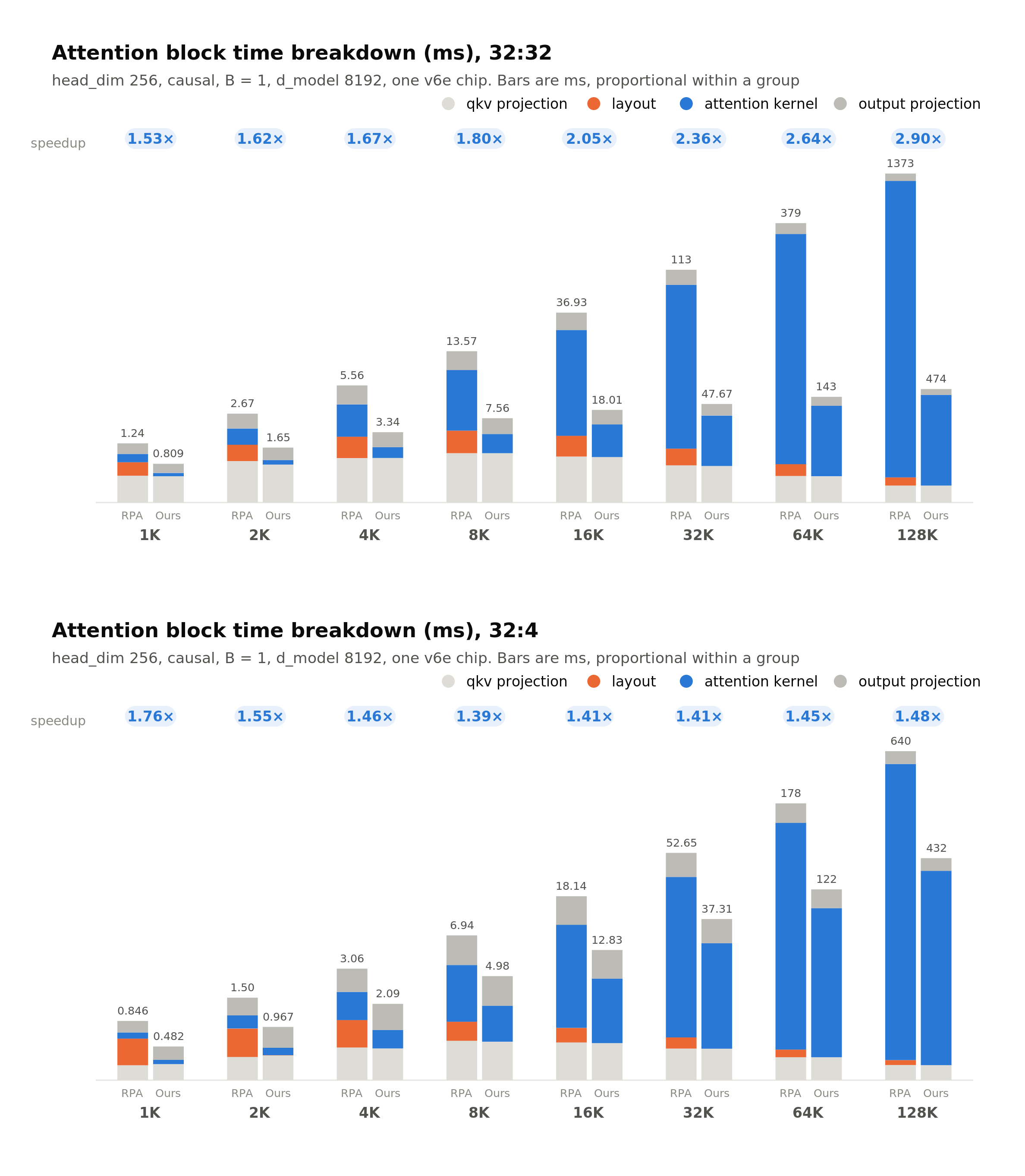
Figure B1. Attention block time on one v6e chip, from hidden states to hidden states, split into the qkv projection, layout, attention kernel and output projection, rpa_v3 vs ours: MHA (top) and GQA with 8 query heads per KV head (bottom).

The layout segment appears only on rpa_v3: under MHA it costs 0.28 ms at 1K and 33.9 ms at 128K, and under GQA it is 45% of rpa_v3’s block at 1K. Ours has none, because the arrangement our kernel needs is absorbed by the projection. Where the gap comes from shifts with sequence length. At 1K, 60% of the MHA gap is rpa_v3’s layout; from 16K on, most of it is the kernel, 75% at 16K and 95% at 128K. End to end, ours finishes a 128K MHA block in 472 ms against 1,373 ms for rpa_v3, 2.9× faster. The ratio grows from 1.6× at 1K because attention grows quadratically with sequence length while the projections grow only linearly: at 1K attention is 3% of the block’s FLOPs, at 128K it is 80%. Under GQA the ratio stays between 1.4× and 1.8×.

References

[1] T. Dao, D. Y. Fu, S. Ermon, A. Rudra, C. Ré. FlashAttention: Fast and Memory-Efficient Exact Attention with IO-Awareness. NeurIPS 2022. arXiv:2205.14135

[2] T. Dao. FlashAttention-2: Faster Attention with Better Parallelism and Work Partitioning. ICLR 2024. arXiv:2307.08691

[3] J. Shah, G. Bikshandi, Y. Zhang, V. Thakkar, P. Ramani, T. Dao. FlashAttention-3: Fast and Accurate Attention with Asynchrony and Low-precision. NeurIPS 2024. arXiv:2407.08608

[4] T. Zadouri, M. Hoehnerbach, J. Shah, T. Liu, V. Thakkar, T. Dao. FlashAttention-4: Algorithm and Kernel Pipelining Co-Design for Asymmetric Hardware Scaling. 2026. arXiv:2603.05451

[5] K. Hong, G. Dai, J. Xu, Q. Mao, X. Li, J. Liu, K. Chen, Y. Dong, Y. Wang. FlashDecoding++: Faster Large Language Model Inference on GPUs. MLSys 2024. arXiv:2311.01282

[6] Z. Ye et al. FlashInfer: Efficient and Customizable Attention Engine for LLM Inference Serving. MLSys 2025. arXiv:2501.01005

[7] S. Yang, Y. Zhang. FLA: A Triton-Based Library for Hardware-Efficient Implementations of Linear Attention Mechanism. 2024. github.com/fla-org/flash-linear-attention

[8] J. Jiang, Y. Chen, B. A. Hechtman, F. Zhang, Y. Mu. Ragged Paged Attention: A High-Performance and Flexible LLM Inference Kernel for TPU. 2026. arXiv:2604.15464

[9] A. Sobczyk, G. Gottardo, C. K. Matzoros, M. De Vita, F. Skogh, A. Zouzias, J. Zhuang. Fast and Stable Triangular Inversion for Delta-Rule Linear Transformers. 2026. arXiv:2605.21325

[10] S. Yang, J. Kautz, A. Hatamizadeh. Gated Delta Networks: Improving Mamba2 with Delta Rule. ICLR 2025. arXiv:2412.06464

[11] S. Yang, B. Wang, Y. Zhang, Y. Shen, Y. Kim. Parallelizing Linear Transformers with the Delta Rule over Sequence Length. NeurIPS 2024. arXiv:2406.06484

[12] SemiAnalysis. TPU Inference Externalization Full Steam Ahead: InferenceX. September 2026. newsletter.semianalysis.com

[13] NVIDIA. CUDA Programming Guide 13.1, Compute Capabilities, Table 30. docs.nvidia.com

[14] NVIDIA. NVIDIA H100 Tensor Core GPU Architecture, whitepaper, Tables 1 and 4. 2022. resources.nvidia.com

[15] NVIDIA. CUDA C++ Programming Guide 12.8, Compute Capability 9.0 and Hardware Multithreading. docs.nvidia.com

[16] NVIDIA. H100 Tensor Core GPU specifications. nvidia.com

[17] NVIDIA. DGX B200 datasheet. resources.nvidia.com

[18] NVIDIA. CUDA Programming Guide 13.1, Asynchronous Data Copies (TMA). docs.nvidia.com

[19] N. P. Jouppi, D. H. Yoon, G. Kurian, S. Li, N. Patil, J. Laudon, C. Young, D. Patterson. A Domain-Specific Supercomputer for Training Deep Neural Networks. Communications of the ACM 63(7), 2020. doi:10.1145/3360307

[20] N. P. Jouppi, S. Lakshmanamurthy, C. Young, D. Patterson. Google’s Training Supercomputers from TPU v2 to Ironwood: Architectural Stability, Scale, Resilience, Power Efficiency, and Sustainability Across Five Generations. IEEE Micro, July/August 2026. arXiv:2606.15870

[21] OpenXLA. Tiled layout. openxla.org

[22] JAX. Writing TPU kernels with Pallas. docs.jax.dev

[23] Google Cloud. TPU architecture, and the TPU v4, v5e, v5p, v6e and TPU7x pages. docs.cloud.google.com

[24] J. Austin, S. Douglas, R. Frostig, A. Levskaya, C. Chen, S. Vikram, F. Lebron, P. Choy, V. Ramasesh, A. Webson, R. Pope. How to Think About TPUs. In How To Scale Your Model. 2025. jax-ml.github.io/scaling-book

[25] P. Toulme. From JAX to VLIW: Tracing a Computation Through the TPU Compiler Stack. December 2025. patricktoulme.substack.com

[26] P. Toulme. When XLA Isn’t Enough, with public LLO compiler dumps for TPU v6e. January 2026. patricktoulme.substack.com, github.com/patrick-toulme/justabyte

[27] JAX. Mosaic TPU vector layout passes, infer_vector_layout.cc and apply_vector_layout.cc, jax-v0.8.0. github.com/jax-ml/jax

[28] NVIDIA. Parallel Thread Execution ISA: warpgroup-level matrix multiply-accumulate (wgmma) and TensorCore 5th generation (tcgen05) instructions. docs.nvidia.com

[29] OpenXLA. Tokamax: Splash Attention for TPU. github.com/openxla/tokamax.

[30] vLLM Project. gdn_v3, the Gated DeltaNet kernel in tpu-inference. github.com/vllm-project/tpu-inference